Following cells through time: my Biohub journey into the bronze range

A microscopy movie is easy to watch and surprisingly hard to understand. Thousands of similar cells move through a developing embryo. Some disappear from view. Others divide. To reconstruct development, we need to follow identities through space and time, not simply find bright spots in individual images.
That was the challenge in Biohub’s Cell Tracking During Development competition. My final selected build reached 0.955 on the public leaderboard and 0.920 on the private evaluation. At the October 1st check, it placed 398th of 4,017 teams: just inside the published bronze range. The medal was awarded by Kaggle when this article was drafted.
Result snapshot · 30 September 2026
Public 0.955 · Private 0.920 · Rank 398 / 4,017
Bronze-range placement.
The problem: follow identities, then recover the family tree
Each timepoint is a three-dimensional image volume. A detection gives a cell centre: where a cell appears at that moment. A link says that one detection and another belong to the same continuing cell. When a parent divides, its lineage branches into two daughters.
The submission is therefore a graph. Nodes represent detections; directed edges represent continuity or division. A cell detector can be excellent and still produce poor tracking if it connects the wrong neighbours. Equally, a good linker cannot recover a cell that never became a candidate.
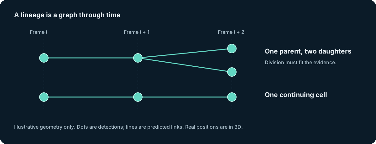
The official evaluation combines adjusted edge Jaccard with a smaller division component: adjusted_edge_jaccard + 0.1 × division_jaccard. This is a tracking metric, not a percentage of cells correctly classified. The sparse annotations and node-count adjustment also make raw graph size an unreliable measure of quality. [1]
A closer look at the real microscopy
The images below come from the competition’s visible sample movie 44b6_0113de3b. The left panel shows one optical plane; the middle takes the brightest value through eleven depth planes. The right overlays predicted cell centres from my saved 84th experiment version 1 output (BH-084). A ring marks a proposed centre, not a segmented cell boundary. Projection makes the volume easier to read, but can superimpose cells at different depths.
.png?generation=1790950126118896&alt=media)
This is a real competition microscopy, frame 0: a single plane, a depth projection and the 84th experiment predicted centres. Predictions are not ground-truth annotations.
Tracking adds identity to those positions. In the next figure, the same colour and number follow one predicted identity through frames 0, 1 and 2. Short lines show its previous projected positions. I selected eight continuing tracks by a fixed rule inside the depth slab, without checking their correctness against labels. These examples explain the representation; they are not an accuracy evaluation or a view of the hidden test set.
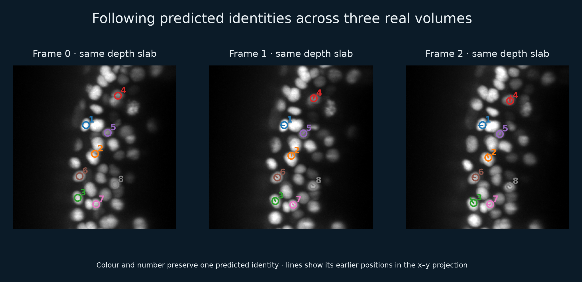
Eight predicted continuing tracks over three real image volumes. All panels use the same depth range and intensity limits; colour and number indicate predicted identity.
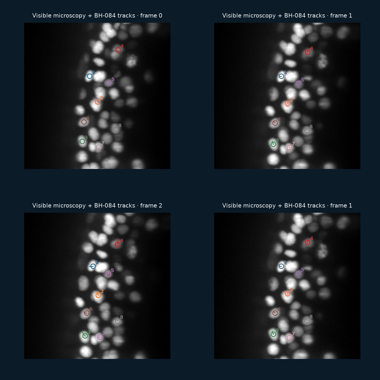
This is the animated view of the same three sample frames and the experiment 84 predictions, playing forwards and backwards. The motion is real microscopy; the overlay is my saved prediction.
How the system learned to see and connect cells
I built on published community notebooks and trained checkpoints. The underlying baseline uses a 3D U-Net with temporal attention to extract visual features and propose cell centres. A transformer then uses features at those centres to score candidate links between successive frames. In the organizer baseline, detection and linking are trained jointly, and only annotated edges contribute to association backpropagation; unannotated cells are not simply treated as background negatives. [2]
A useful way to picture learning is a repeated comparison: the model proposes a connection, training labels supply evidence about the correct connection, and optimization adjusts the model’s weights. After training, those weights turn new image volumes into predictions. The hidden competition labels are unavailable to us.
My final notebooks loaded existing learned checkpoints. The final push was primarily about inference and graph construction, rather than training a new detector from scratch. I did explore learned temporal and division-related challengers earlier in the campaign, but a promising result on one embryo did not automatically earn integration: some failed when tested in the opposite transfer direction.
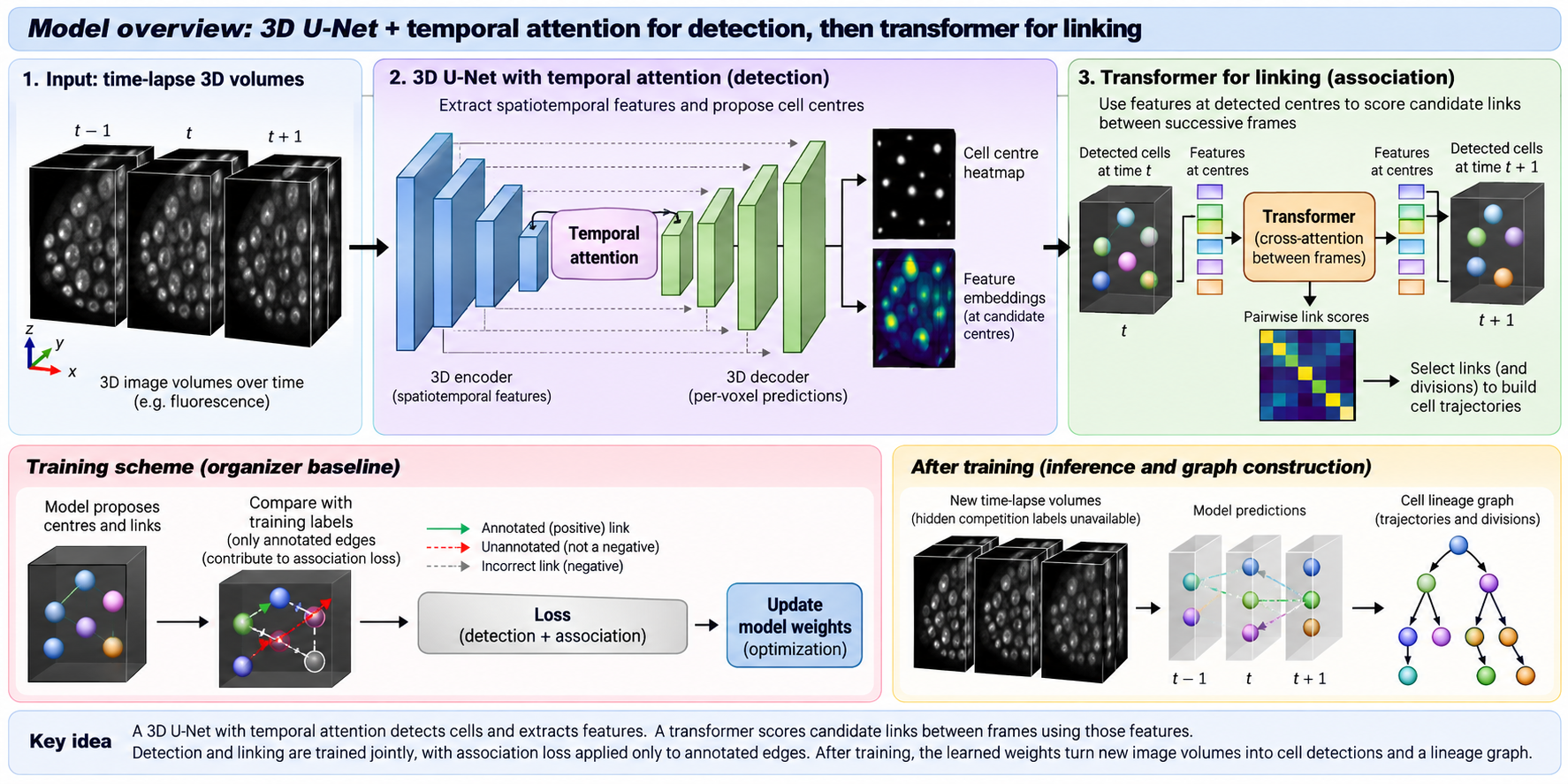
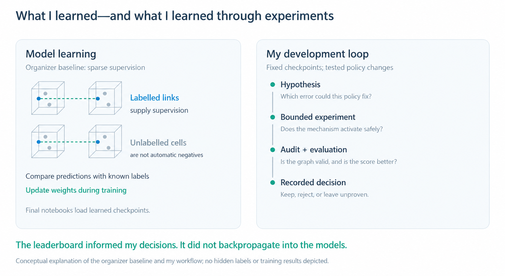
Two feedback loops: sparse supervision trains the model; tests and scores guide our experiment decisions. This is a conceptual schematic, not a training result.
From probabilities to a consistent lineage
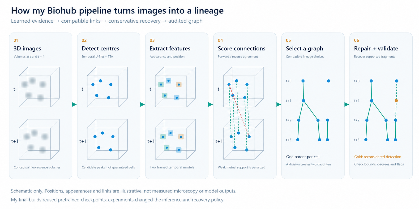
My pipeline shown as image volumes, cell centres, feature evidence, competing links and a repaired lineage. All positions are just illustrative.
The inherited inference stack used two temporal models and spatial test-time augmentation. Looking at transformed views can stabilize predictions, but more views are not guaranteed to help: I tested alternatives and recorded regressions as well as improvements.
I also evaluated a candidate connection in both temporal directions. Does the earlier cell support the later cell, and does the later cell support the earlier cell? Weighted harmonic fusion penalizes a connection when either direction provides weak support. It turns mutual agreement into evidence; it does not make agreement proof of correctness.
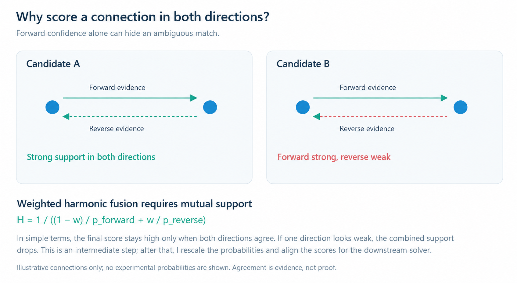
A connection supported in both directions differs from a forward-only confident match. The formula illustrates the intermediate fusion, before normalization and logit alignment.
A constrained graph solver then selects a compatible set of links instead of taking each highest probability independently. The surrounding policy checks temporal direction, lineage degrees and plausible geometry. Conservative repairs can recover missing detections or bridge gaps, while auxiliary centre evidence helps veto unsupported additions. Runtime limits and fallback flags make operational failures visible.
The changes that shaped my final builds
Experiment 70 (BH-070) combined two recall adjustments that I had first scored separately: lowering the main detection threshold to 0.960 and allowing nearby discarded peaks back into consideration at 0.950. It reached a reported public score of 0.955 and became my preferred experiment.
The final alternative, Experiment 80 (BH-084), used detection threshold 0.9575 and readmission threshold 0.945. These numbers govern different decisions. Raising the detection threshold demands stronger initial evidence; lowering the readmission threshold allows more nearby candidates to be reconsidered. Their joint effect must be measured, because changes can overlap or interfere.
I chose experiments 70 and 84 (BH-070 and BH-084) as my two final submissions (out of 85 experiments) before seeing the private scores. Both were completed, audited and graph-distinct. I retained the incumbent and one interaction alternative rather than assume a displayed public tie meant identical behaviour.
| Experiment | Detection threshold | Readmission threshold | Public score | Private score |
|---|---|---|---|---|
| BH-070 | 0.960 | 0.950 | 0.95593 | 0.91896 |
| BH-084 | 0.9575 | 0.945 | 0.95552 | 0.92015 |
On the private evaluation, BH-084 was better by 0.002 at the reported precision. This does not identify which threshold caused the difference, nor prove that the recipe will win on another dataset. It does show that my distinct alternative mattered in this competition.
Trial and error, with a memory
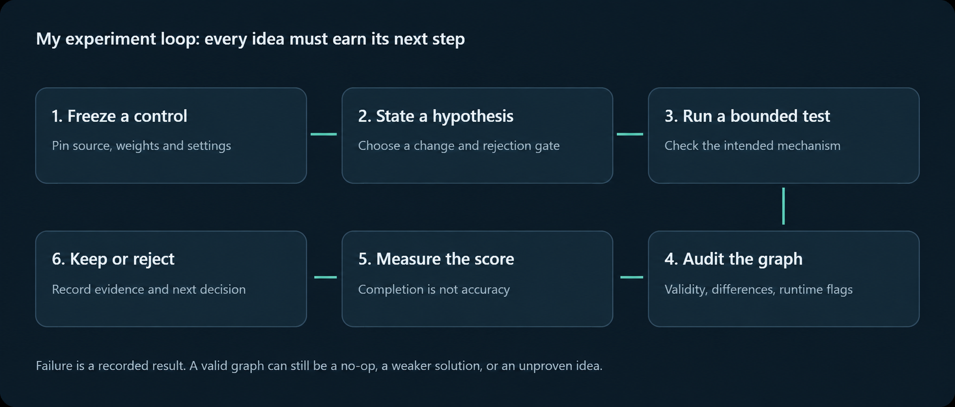
A bounded experiment earns a score slot only after its implementation and output pass the relevant gates.
The campaign was a sequence of explicit hypotheses, frozen controls and receipts. Each experiment had a name, a source lineage and a decision. I pinned notebook versions and artifact hashes, saved runtime statistics, compared graphs at coordinate level and recorded actual Kaggle submission IDs. A completed notebook was an artifact; a completed competition evaluation was score evidence.
I used tests to establish that a policy did what it claimed, and audits to establish that the output was a valid graph. Neither establishes accuracy. Where local validation was available, I examined transfer across embryos and sequence-level failures, rather than rely only on one favourable aggregate.
One instructive failure was BH-082. It aimed to recover very short three-frame tracks under strict evidence requirements. The graph was valid, but the intended three-frame rescue count was zero. I excluded it from scoring under the declared mechanism gate. That saved a submission slot and prevented a no-op hypothesis from being presented as a successful experiment.
Other ideas did activate. BH-081 recovered 83 short-track nodes across 18 components; BH-083 selected 68 motion-supported candidates. Those counts showed that the mechanisms ran. They did not show that the added cells were correct. Both ultimately reported 0.955 publicly, illustrating how substantial graph changes can leave a rounded leaderboard score unchanged.
Where AI assistance fitted into the work
I used Codex to help implement bounded changes, inspect failures, build notebooks, run focused checks and maintain the experiment ledger. That assistance via my own skill files made it practical to keep provenance and rejection decisions alongside the code. The scientific decisions still depended on measured evidence and the compute and submission budget (30h of GPU compute a month plus an plus OpenAI subscription using chat GPT 5.5).
There were two distinct feedback loops: trained neural networks learned from labelled examples; my development process learned which hypotheses survived tests, audits and evaluation. A leaderboard submission supplied evidence for the next decision (it did not itself backpropagate into the model).
What took me into the bronze range
There was no last-minute public-score breakthrough. My final-day candidates did not exceed the reported 0.955 ceiling, and GPU quota ran out. Two additional ideas were built and locally tested but never run on the full test set, so I kept them ineligible rather than describe them as improvements.
The result came from the accumulated pipeline, careful recall policies, valid execution and a useful final alternative. At 398th of 4,017 teams, my placement was three positions inside the nominal bronze cutoff of 401. That is a narrow result. [3]
The lesson I would carry into the next competition is to make every experiment answer a question. A failed mechanism, a broken evaluator and a weaker score are useful when they are recorded honestly. They tell us where to stop, which assumptions need repair, and where the next unit of compute is most likely to teach us something.
I had spent two months on this competition, day and night and, it was fun. I take a lot of lessons learned.
Credits and sources
This work stands on the organizer’s tools and community contributions, rather than a wholly original architecture. Our recorded lineage includes Harmonic Fusion notebooks, Anvith Pothula’s coordinate-refinement work, Yusuke Togashi’s mutual-support fusion rule, and the public model/support datasets published by pilkwang. Earlier reproduced controls also credited Yunus Gumsoy, Rishabh Roy, flexonafft and Reyhan K. Satria. Source attribution and license checks were retained in the experiment records.
- Get link
- X
- Other Apps
%20applied%20to%20Transformer%20models%20in%20machine%20learning.%20The%20image%20shows%20a%20neural%20networ.webp)

Comments
Post a Comment